In this post we will talk about some of the data-structure issues that arise in algorithms for dynamic connectivity.
When talking about dynamic algorithms, we skipped over the details of the underlying data structures. These data-structures are interesting objects in themselves, so let me say a few words. The material below is supplementary material (I will not test you on this), but it answers questions raised in lecture, and may be fun for some of you.
Frederickson’s $O(m^{2/3})$ algorithm
Implementing Frederickson’s algorithm did not require any fancy data structures. For each edge, we maintain whether it belongs to the spanning tree. For each node $v$, we remember its incident edges, and a pointer to the cluster $v$ belongs to. For each cluster we maintain a pointer to the tree it belongs to.
When an edge $(u,v)$ is added, we look up the containing clusters $C_u, C_v$ for the endpoints, and then look up the trees $T_u, T_v$ containing those clusters. This takes $O(1)$ time. Now if the endpoints lie in different trees, we mark this edge as a spanning-tree edge (in $O(1)$ time), and change the name of the containing tree for each of the $O(m/z)$ clusters in the combined tree (in $O(m/z)$ time). If needed, the clusters $C_u$ and $C_v$ are merged with adjacent clusters (and repartitioned) so that the clusters have size in $[z,3z]$. This takes another $O(z)$ time. The edge deletions can also be done in class using these elementary operations.
A Data Structure to Maintain a Changing Forest
However, for the other algorithms we briefly discussed, we need a bit more sophistication. So let’s imagine we have a data structure that maintains a forest (i.e., a collection of rooted trees), and supports the following operations:
- Createtree(v) makes a new single-node tree $v$ and adds it to the forest.
- Findroot(v) returns the name of root of the tree containing $v$.
- Cut(u,v) takes an edge $(u,v)$ in some tree $T$, and deletes this edge, thereby giving two new trees. If $u$ is the parent of $v$ in the rooted tree $T$, then $v$ becomes the root of its tree.
- Link(u,v) takes two nodes $u, v$ from different trees, and connects them using a new edge $(u,v)$.
- Weight(r) takes a root node $r$, and returns the sum of weight of the nodes in the tree rooted at $r$.
- AddWeight(v, c) adds $c$ to the weight of a node $v$.
(Here we imagine the weights are elements of some commutative group.) Note this this data-structure works only when the set of edges are acyclic, so it will help us maintain and update the spanning forest that all the algorithms maintain.
Using these Operations for our Algorithms
We now discuss how to use this data-structure for our dynamic connectivity algorithms. Later we will discuss how to implement such a data-structure.
The Kapron, King, and Mountjoy Algorithm
We just talked about a single edge-deletion and finding a replacement edge. Clearly, deleting the edge $e = (u,v)$ is easy using the cut operation. Two other non-trivial operations were to find the fingerprint of a tree, and to check if there was a false positive (which was Corwin’s question). Let’s consider these one by one.
Remember the label of each edge was just the $2\log n$-bit tuple of the names of its endpoints, the label of a node was the bit-wise XOR of the labels of all its incident edges, and the fingerprint of a tree was a bit-wise XOR of the labels of all the nodes in the graph. We can think of the weight of a node as being its label. Since the set of bit-strings under bit-wise XOR form a commutative subgroup, operation $4$ allows us to find the total weight of the tree, which is its fingerprint! (Moreover, on deleting $(u,v)$ we can change the weight of $u$ and $v$ using the AddWeight operation.
Moreover, if the fingerprint $(u’,v’)$ happens to be a false-positive, i.e., it is not an edge connecting the subtrees $L,R$ formed from $T$ by deleting the edge $e$, we can figure this out by running Findroot with $u’$ and $v’$, and checking if these are the same as Findroot(u) and Findroot(v).
The Holm, de Lichtenberg, and Thorup Algorithm
We talked about this very briefly, so I’ll say only a few words. The Weight operation makes it easy to figure out which side has the smaller number of nodes, and then we can alter the levels of edges on that side. We will need to maintain extra information to iterate over just the edges having a particular level, but I will not get into this here. Instead let us talk about how to implement the data-structure described above.
How to Implement such a Data Structure?
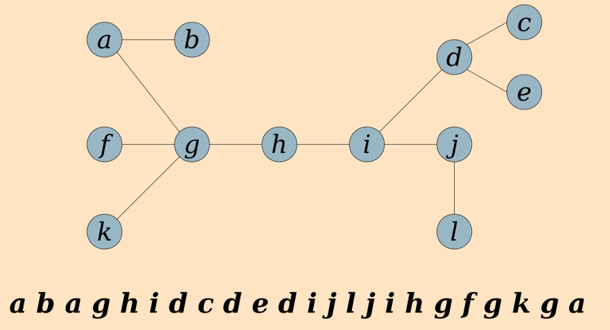
The implementation I will talk about is a paraphrasing of the well-known Euler-Tour trees of Monika Henzinger and Valerie King. Their idea is to represent each tree $T$ as its Euler tour, starting and ending at the root. This is a list of length $2|V(T)|-1$. Note that each vertex appears multiple times in the list. E.g., see below (figure from Keith Schwarz’s excellent slides):
For the moment, let’s not worry about the low-level implementation details, and just imagine how we’d like to ideally implement each of the operations above.
-
Createtree(v) just creates a new Euler tour with a single node v.
-
Findroot(v) returns the first (= last) element in $v$’s Euler tour.
-
Cut takes the Euler tour for the tree containing $u,v$. Now it finds where $(u,v)$ and its reverse direction $(v,u)$ are traversed in the Euler tour. It now splits the Euler tour into three parts at this position: that from the root until visiting u, the part starting and ending at v, and the rest starting at u and ending back at the root. If we merge the first and third part, we get the Euler tours for the two trees!
-
Find is the exact opposite of the above operation. If $v$ were the root of its tree, we would find some occurrence of $u$ in its Euler tour, split the list there and insert the tour for $v$ there. (If $v$ is not its tree’s root, we can re-root it as follows: find the first occurrence of $v$ in its tour, cut out the portion of the tour before this occurrence and attach it to the end, so that we start and end at $v$.)
-
Hmm, how to maintain weights? Let’s see a bit more detail how to implement these operations a little more in detail first.
Removing Another Layer of Abstraction
To implement the operations above, we need to maintain lists: to find the first position of an element in a list, to cut a list at any point, and to join together two lists, ideally all in logarithmic time. If we imagine the list to be elements in a dynamic binary search tree (such as a Splay tree or a red-black tree), we can do all these operations seamlessly, with $O(\log n)$ update times.
Finally, what about the weights? This is easy: for each node in the binary search tree (BST), just maintain the weights of the elements in the subtree under it. Then, since the (average) depth of nodes in such a BST remain small, updating the weight of the subtrees can also be done fast, by updating the weights on the path from the updated node all the way to the root.
Further References
You can look at the original paper on Euler-Tour trees for ET-trees for more details. A very related data-structure is link-cut trees of Danny Sleator and Bob Tarjan. Finally, the slides from Stanford’s CS166 give a good explanation of the Holm et al. algorithm, for those of you wanting to learn more.