The Expert Weights, and the Zero-Sum Game view
Pedro asked for some intuition for how these probabilities were evolving. Well, they’re playing the role of the dual variables (and averaging them can indeed give the duals). But I find it cleaner to view them in the zero-sum game view.
The Cut-Flow Game
One way to view the max-flow problem is as a zero-sum game. The row (or cut) player Clara picks a random edge, and the column (or flow) player Fred picks a random $s$-$t$ path. The payoff to the row-player Clara is $1$ if the edge she picks lies on the path picked by the column player, and is zero if her edge does not lie on the path. Assume the maximum $s$-$t$ flow is $F$
Observation: the row player can guarantee she gets a payoff of at least $1/F$. Why? She can choose any min-cut (which by max-flow min-cut equals $F$), and pick one edge from this cut uniformly at random. Then no matter what path is picked, this random edge lies on that path with probability at least $1/F$.
Observation: the column player can guarantee that the payoff to the row-player is at most $1/F$. How? He can fix a max-flow of $F$, and imagine that this flow can be decomposed as $\sum_P f_P$, where $f_P$ is the amount of flow on the $s$-$t$ path $P$. Now here’s a strategy for the column player: he picks a random path $P$ with probability $f_P/F$. Given this strategy, the row-player’s optimal strategy is to pick the edge with the highest payoff $\sum_{P: e \in P} f_P/F$. But because we respect edge capacities, $\sum_{P: e \in P} f_P \leq 1$ and hence the payoff is at most $1/F$.
Hence one way to solve the zero-sum game is for the row-player to compute the min-cut and the column-player to compute the max-flow. Since MW solves zero-sum games, let’s see what it does.
The Experts-Based Algorithm
Now you can view the algorithm we gave as just using the zero-sum games algorithm from the previous lecture. The row-player uses Hedge to update the weights, the column player plays best-response. Finally, you can take the row-player’s empirical average $\hat{x} := \sum_t p^t$ and the column-player’s empirical average $\hat{f} := \sum_t f^t$. These are almost optimal (minimax) responses to each other. Hence, $\hat{f}$ will converge to a max-flow, and $\hat{x}$ will converge to a (fractional) minimum cut. In other words, the $p^t$ values (averaged) are acting like the minimum cuts.
The Name of the Game: Controlling the Width
The reason why we went from using shortest paths to using electrical flows is all to do with the width. Let me say some more. Recall that for the analysis of Hedge, we said that if the “gain” (or “loss”) vectors are bounded in $[-\gamma, \rho]$, then the time to get the average regret down to $\varepsilon$ is
The quantity $\max{\rho, \gamma}$ is called the width of the problem. To solve LPs, the $i^{th}$ coordinate of the gain is set to be he violation of the $i^{th}$ constraint. For the path-based LP we use for the max-flow problem, each constraint corresponds to an edge. And the violation of the edge $e$ is $f_e - 1$, the flow on edge $e$ minus its (unit) capacity. Since we route all the flow on a single path, this quantity belongs to the set ${-1, F-1}$, so the convergence time is $O(F \log m/\varepsilon^2)$. And $F$ may be as large as $\Omega(m)$.
The use of the electrical flows uses fact that the amount of flow on any edge is at most $O(\sqrt{m})$. This is true at the beginning, when all the resistances are $1$, but later (if we set $r_e = p^t_e$) this may not be true: if some edge has some tiny probability, its resistance may be close to zero, and hence we may send almost all the flow on it. To control that, here’s a cute trick. Set the edge resistances $r_e := p^t_e + \varepsilon/m$. Now the same analysis as in lecture shows that the flow on any edge is at most $\sqrt{m/\varepsilon}$! (All this is in the lecture notes.) So we’re using a different algorithm to solve the average problem, one which has much better width.
Sarthak had a good question: don’t we need to show that the electrical flow actually satisfies the average problem? Indeed we do, I completely forgot to show that in lecture. The proof is easy, though. If we set $r_e := p^t_e + \varepsilon/m$, the max-flow $f^\star$ has energy burn $\sum_e (f^\star_e)^2 r_e \leq (1+\varepsilon)$. So the electrical flow $f$ has at most as much energy burn, i.e., $\sum_e f^2_e r_e \leq \mathcal{E}(f^\star) \leq (1+\varepsilon)$. Now using Cauchy-Schwarz, we get
So we’re (approximately) solving the average problem. If you work through the calculations, the $\varepsilon$ loss here can be absorbed in all the other losses.
A Tight Example for the Basic Electrical Flow Algorithm
So is the width of this electrical flow algorithm actually $\Omega(\sqrt{m})$, or is the algorithm good and we just need a smarter analysis? Here’s an example from the Christiano et al. paper that shows that the width of the basic electrical flow oracle can be as large as $\sqrt{m}$, with all edges having unit resistance.
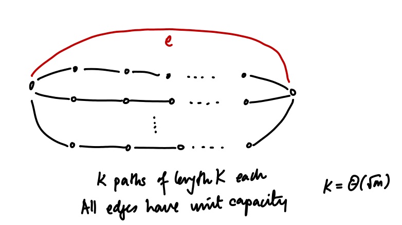
The effective resistance of the entire collection of black edges is $1$, so half the current flows on the top red edge. If we set $F = k+1$ (which is the max-flow), this means a current of $\Theta(\sqrt{m})$ goes on the top edge. Hence the width.
The Improved Electrical Flow Algorithm
How does one do better? The idea is clever but simple. Make the width small by force. If you find the electrical flow and the flow over some edge $e$ is more than $\approx m^{1/3}$, just delete that edge. Now, by construction, the width is $\approx m^{1/3}$. However, now we’re changing the structure of the proof. The worry is that the max-flow may go down if we delete edges. What if we end up deleting all the edges? Thankfully, the proof (also in the old lecture notes) shows that we delete only an $\varepsilon F$ number of edges, so things are controlled.
And here’s another example (via Gary, who got this one from Olek Madry) that shows that the fancier algorithm does need $\Omega(m^{1/3})$ iterations, and does need to delete $\Omega(m^{1/3})$ edges.
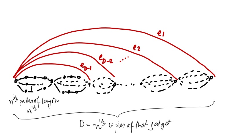
Again, in this example, $m = \Theta(n)$. And again, each black gadget has a unit effective resistance, and if you do the calculation, the effective resistance between $s$ and $t$ tends to the golden ratio. If we set we set $F = n^{1/3}$ (which is almost the max-flow), this means a constant fraction of the current, or about $\Theta(n^{1/3})$ goes on the edge $e_1$. Once that is deleted, the next red edge $e_2$ carries a lot of current, etc. Until all red edges get deleted.
The Example from Lecture
Some of you asked me for more details about the example, to understand how it would evolve. For that, let’s consider a generalization of the example we did in lecture.
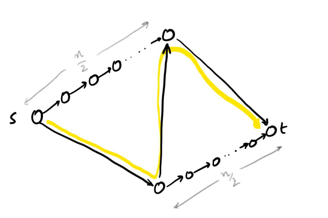
The max-flow is $F = 2$, using the two straight paths. But the zig-zag path (highlighted) only uses three edges, as opposed to the $n/2$ for the straight paths, so at the start the Hedge-based algorithm really prefers the zig-zag path. But eventually, whatever Hedge does, if we want the flow to be $(1+\varepsilon)$-approximate, only $O(\varepsilon)$ of the flow should use the zig-zag path. And hence, after some time, most of the paths the algorithm finds should be the straight paths. Let’s see why that’s the case.
For simplicity, assume that the length of an edge is $e^{\varepsilon \cdot \text{load}}$. (The actual lengths are $e^{\varepsilon \cdot \text{(load} - \text{number of iterations)} }$, but dropping the $e^{- \varepsilon \text{number of iterations}}$ term from every edge does not change anything, and makes the calculations easier.)
Consider the situation after some iteration $t$. We’ve sent $2t$ units of flow so far, since we send $F = 2$ units per iteration. Say $\delta t$ of the iterations chose the zig-zag path. The load on the top-right and bottom-left edges is $(1+\delta)t$, so their lengths are $e^{\varepsilon (1+\delta)t}$. The lengths of all other edges on the top and bottom are $e^{\varepsilon (1-\delta)t}$. We’ll ignore the length of the vertical edge to make things simple — it’s not really crucial.
Consider time $T = \Omega(\log m/\varepsilon^2)$, the length of the top left path is $n e^{\varepsilon (1-\delta)T}$. This is $\leq e^{\varepsilon (1+\delta)T}$ if $\delta \geq \varepsilon$. So anytime after time $T$, if $\gg \varepsilon$ fraction of the total flow is on on the zig-zag path, we’ll be sending flows on the straight paths and thereby correcting this situation. Indeed, this ensures that the average flow is at most $(1+\varepsilon)$ on all edges after $\Theta(T)$ time.